What is a place, to a model that has never seen a thermometer?
AlphaEarth Foundations reads a year of Sentinel-2 imagery and returns 64 numbers for every 10 m cell of the planet. This is an atlas of what those numbers know about Europe, and a pre-registered test of whether they beat hand-crafted covariates at downscaling temperature. They did not.
The pre-registered result
Predicting COSMO-REA6 daily maximum temperature at 6 km from ERA5, the embeddings reach an RMSE of 1.530 K, compared with 1.469 K for a stack of hand-crafted covariates: elevation and its roughness, slope and aspect, distance to coast, impervious and tree fraction, population density, and built height. That is 4.2% worse on RMSE and 4.3% worse on CRPS, pooled over 5 held-out spatial folds. The decision rule asked for a 10% improvement in the other direction and was registered, with the fold assignment hashed, before any probe was fitted.
Adding the embeddings to the covariates recovers almost nothing (1.467 K compared with 1.469 K), which is the more informative half of the result: whatever the embedding knows about a 6 km cell of Europe, elevation and a coastline distance already knew. The six-arm table is in Methods.
Act 1
The Continent, Sorted
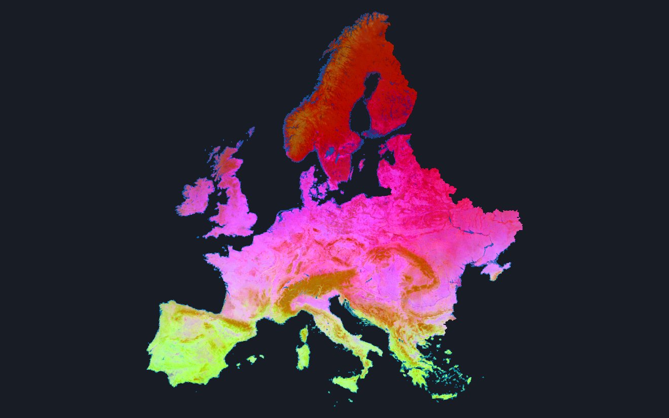
Each embedding is a 64-dimensional unit vector, so a cell's information is a direction rather than a magnitude. Pooled onto the COSMO-REA6 6 km grid and projected onto the first 3 principal components of that pooled cloud, the direction becomes a colour. No temperature, elevation, or coastline enters the projection.
What comes out is still a map of Europe. The Alps separate from the Po valley, the Iberian meseta separates from the Atlantic fringe, and the boundary between coast and interior is drawn without anyone naming a coast.
Act 2
Temperature Without a Thermometer
Correlate each projected axis against mean JJA daily maximum temperature and the second component reaches r = +0.688, with a block-bootstrap 95% confidence interval of [+0.643, +0.730] over 234 spatial blocks. The signal is on PC2. PC1 measures -0.195, which is weak and the wrong sign, so the signal is not on the embedding's first component.
The bootstrap resamples 33-cell blocks rather than cells, because a climate field is autocorrelated and a cell-wise interval on 150,559 cells would be far too narrow to mean anything. A partial correlation controlling for latitude and elevation gives -0.204, so most of what PC2 carries at this resolution is geography the covariate stack already has.
Act 3
Nine Years of a City
Tier B demonstration. This panel is 10 m urban texture. It is not validated temperature, and nothing here has been through the spatial block cross-validation that produced the result at the top of the page.
Paris and Madrid, 2017 to 2025, 18 rendered units per city. One channel is the embedding itself on the same 3 components as Act 1. The other is the angle between one year's embedding and the next, which is where change appears.
Most of what lights up is agriculture. In the naive year difference the Paris cropland control moves 50.92 degrees between consecutive years, compared with 16.66 degrees at the construction site, so a ploughed field is the brighter object. The one place named as construction here is the Village des Athlètes at Saint-Denis. The Madrid inset is an irrigated-belt parcel, a candidate rather than a labelled site.
A persistence filter was built to separate lasting change from crop rotation, and it did not clear its pre-declared gate. The control's persistence score came out at 0.291 of the construction site's, where the gate required 0.25 or less. 3 of the four criteria passed. The filter is not shipped, the naive difference is what is drawn, and the failure is stated rather than tuned away. The four criteria and what each measured.
Act 4
Norms and the Cost of Pooling
Every embedding leaves the model on the unit sphere, so pooling 10 m cells to 6 km by plain averaging shortens the vector, and it shortens it unevenly. Across the pooled grid the coefficient of variation of the norm is 9.01% against 1.26% at native resolution, and the pooled median norm is 0.8726 of the native one. The norms ship as int8 ratios against one shared reference, so ratios and coefficients of variation are quotable here and an absolute radius is not.
Averaging inside a 6 km cell contracts a heterogeneous neighbourhood towards its own mean direction, so the contraction factor becomes a proxy for how mixed the cell is, entangled with the direction that carries the meaning. The arm that turns this from a story into a diagnosis is MOSAIKS. Random convolutional features are built to be spatially averaged, so pooling is a valid operation on them, and MOSAIKS lands at 1.480 K where the embeddings reach 1.530 K. The narrower reading of the headline is that mean-pooling a hypersphere embedding to 6 km is the wrong operation, and a random-feature baseline that tolerates pooling gets closer to the covariates than the foundation model does.